Equations used in the solvers
Shallow-water equations
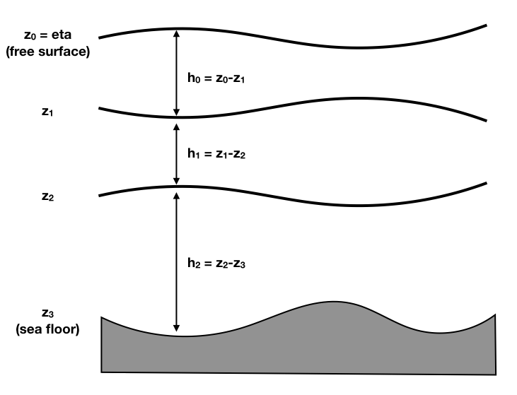
We consider a layered ocean with upward oriented z-axis:
The adiabatic and non-dissipating shallow water equations for \(N\) layers can be written as
for \(n=0,\cdots, N-1\) (\(n=0\) corresponding to the top layer) and where \(\mathbf{u}_n\) and \(h_n\) are the layer 2d velocity and thickness, respectively, and \(g\) is the gravitational acceleration.
The normalized Montgomery potentials \(m_n = M_n / (g\rho_n)\) are proportional to the Montgomery potentials \(M_n\) and can be computed as \(m_0 = z_0\) and, for \(n>0\), as
Here \(\rho_n\) is the density in layer \(n\) and \(z_n\) is the \(z\)-coordinate of layer \(n\) upper boundary, given by:
For example for \(N=2\), \(z_0 = - H(\mathbf{x}) + h_1 + h_0\) and \(z_1 = - H(\mathbf{x}) + h_1\). The total depth can be decomposed as the sum of a constant “full depth” \(\tilde H\) and a topography \(T(\mathbf{x})\) (the height of the submarine mountains), \(H(\mathbf{x}) = \tilde H - T(\mathbf{x})\), so that we find
The equation for normalized Montgomery potential may be rewritten into a useful equation for interface vertical position:
Note that since the velocity fields \(\mathbf{u}_n\) are not divergent-free, we have \(\mbox{D}_t \mathbf{u}_n = \partial_t \mathbf{u}_n + \boldsymbol{\nabla} |\mathbf{u}_n|^2/2 + \zeta_n \mathbf{e_z}\times \mathbf{u}_n\), with \(\zeta_n = \mathbf{e_z} \cdot (\boldsymbol{\nabla} \times \mathbf{u}_n )\) the relative vorticity.
Considering now Earth rotation, forcing, and, dissipating terms, the shallow water equation for conservation of momentum can be written as:
for \(n=0,\cdots, N-1\) and where:
\(f\) is the Coriolis frequency,
\(\Pi_n\) is a forcing potential, presumably tidal,
\(\mathbf{F}_{un}\) gathers non potential forcing (typically relaxations),
\(\mathbf{D}(\mathbf{u}_n)\) is dissipation.
The thickness tendency equation is:
where \(F_{hn}\) represents thickness forcing and/or diabatic effects.
The pressure can be recomputed as:
The one-layer case for N=1 is implemented in fluidsim.
Conserved quantities
We need to write the formula for the main quantities conserved by the equations.
kinetic energy:
potential energy:
available potential energy:
where \(\eta_n\) is the departure of the n’th interface from its position at rest.
potential enstrophy:
Note that the potential vorticity is \(q_n=(\zeta_n+f)/h_n\)
Vertical normal modes
We assume now the layers are weakly departing from a rest state characterized by layer thicknesses \(H_n\) and associated interface vertical positions \(Z_n\). We also assume the topography is flat. Interface displacement from their positions at rest are labelled \(\eta_n\), such that:
The temporal evolution of layer thicknesses is then given by:
One can then separate vertical and horizontal dependencies according to:
The vertical mode structure functions \(\phi_n\) satisfy the following eigenvalue problem:
for \(0<n<N-1\), and:
The eigenvalue if related to an equivalent speed \(c_n\) according \(c_n=\sqrt{g/\lambda}\)
Quasi-geostrophic equations
We consider now that the flow weakly depart from a reference state given by constant and uniform layer thicknesses \(H_n\).
Each interface is departing from its mean position by \(\eta_n\). The layer thickness is then given by \(h_n=H_n+\eta_{n}-\eta_{n+1}\).
Normalized Montgomery potentials anomaly are then given by \(\mu_0 = \eta_0\) and for \(n>0\) as:
This last expression can be rewritten to express \(\eta_n\) as a function of \(\mu\)’s:
where the last approximation will be considered as an equality next.
Under typical quasi-geostrophic conditions (weak Rossby number, weak topography), the flow is at zeroth order geostrophic:
The geostrophic streamfunction is thus \(\psi_n=g \mu_n/f_0\).
The curl of momentum conservation is at first order given by:
where \(f'=f-f_0\).
The divergence of the horizontal flow is given by the thickness tendency equation:
which leads to the conservation of QG potential vorticity:
where \(q_n\) is the quasi-geostrophic potential vorticity:
For interior layers (\(0<n<N-1\)):
where \(g_n'=g(\rho_n - \rho_{n-1})/\rho_n\).
Forcing: waves
We want to force internal waves with a given frequency \(\omega\) and modal vertical structure corresponding to mode f. The forcing required to do that, while not producing spurious QG potential vorticity, should look like:
where (\(f_u\), \(f_v\)) are constants, \(h(x,y)\) describes the horizontal spatial and temporal structure of the forcing, \(\phi_f\) is the \(f\) vertical mode number. The spatiotemporal structure is chosen to match that of the expected wave, i.e. a sinusoidal-like shape with wave number \(k\) satisfying the following dispersion relationship
In general: \(h=\sin[ k (y-y_c)-\omega t]\)
A dirac in y and spatial uniformity in x may also work.
Forcing: vortices
In order to force a turbulent eddy field, we apply a forcing that looks like:
where the spatial and temporal structure of the forcing is given by:
where \(s\) is a smoothly varying step function. The QG potential vorticity will be generated at the following rate:
We choose for now \(f_{uv}=0\).